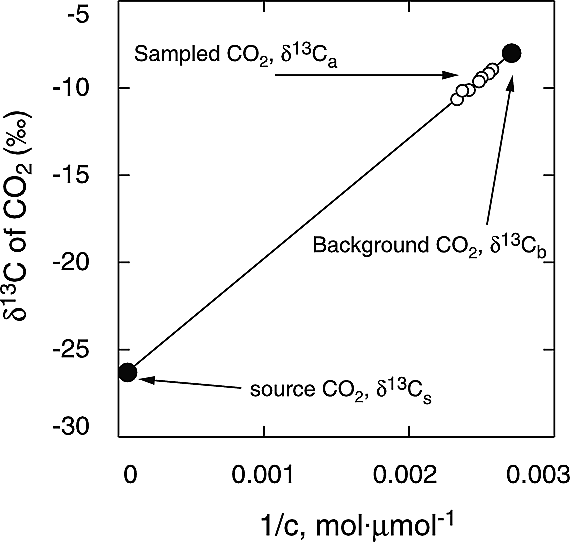
Pataki (2003) Figure 1. Graphical illustration of the Keeling plot method given as equation (3) in the text. The carbon isotope composition of two endpoints of source CO2 (δ13Cs) and well-mixed, background atmospheric CO2 (δ13Cb) are shown in solid circles. The carbon isotope composition of sampled air (δ13Ca) is shown by open circles. Isotope ratios are plotted against the inverse of CO2 concentration (c). Note the distance of the samples from the intercept.
C_added = amount of “source” CO2 added to the atmosphere (also called C_s)
C_old = initial (“background”) amount of CO2 in the atmosphere (also called C_b)
C_new = the observed amount of CO2 in the atmosphere after the addition (also called C_obs)
F_added = isotopic composition of added CO2 (also called δ_s)
F_old = isotopic composition of original atmosphere (also called δ_b)
F_new = isotopic composition of atmosphere after the addition (also called δ_obs)
Note: Keeling plots are most often used with δ13C data, but are not restricted to that.
The Keeling Plot is F_new (on the Y-axis) vs (1/C_new) on the X-axis.
The slope is: 𝑑 F_new / 𝑑 (1/C_new)
which is: C_old ⋅ (F_old − F_added)
The Y-intercept is where (1/C_new) is zero, so F_new = F_added.
So you can plot the F_new (measured atmospheric isotope fraction) on the Y-axis
vs. 1 over C_new (reciprocal of the measured CO2 level),
and extend the slope back to X=0,
and read the F_added (isotope fraction) from the Y-intercept.
Note: In the real world, carbon emissions into the atmosphere come from many sources, with varying δ13C
levels. What's more, there are not only emissions, there are also very large exchanges of carbon between the atmosphere and
other “carbon reservoirs,” such as the oceans and the terrestrial biosphere & soils, all of which also affect
atmospheric CO2 isotope ratios. Like everyone's favorite Facebook “relationship status,” it's complicated.
Pataki, D. E., et al. (2003). The application and interpretation of Keeling plots in terrestrial carbon cycle research. Global Biogeochem. Cycles, 17(1), 1022, pp. 1-14. https://doi.org/10.1029/2001GB001850